NumPy
![]()
NumPy, which stands for Numerical Python, is a free, open-source Python library for working with arrays. It's one of the most popular packages for scientific computing in Python, and is used for data manipulation and analysis, including data cleaning, transformation, and aggregation.
- Official Website: https://numpy.org/
- Installation: (https://numpy.org/install/)
pip install numpy
- Documentation: https://numpy.org/doc
- GitHub: https://github.com/numpy/numpy
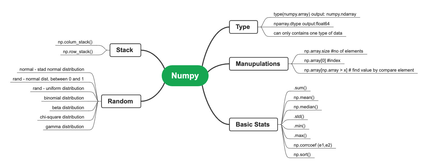
📊 Click to view NumPy Mindmaps
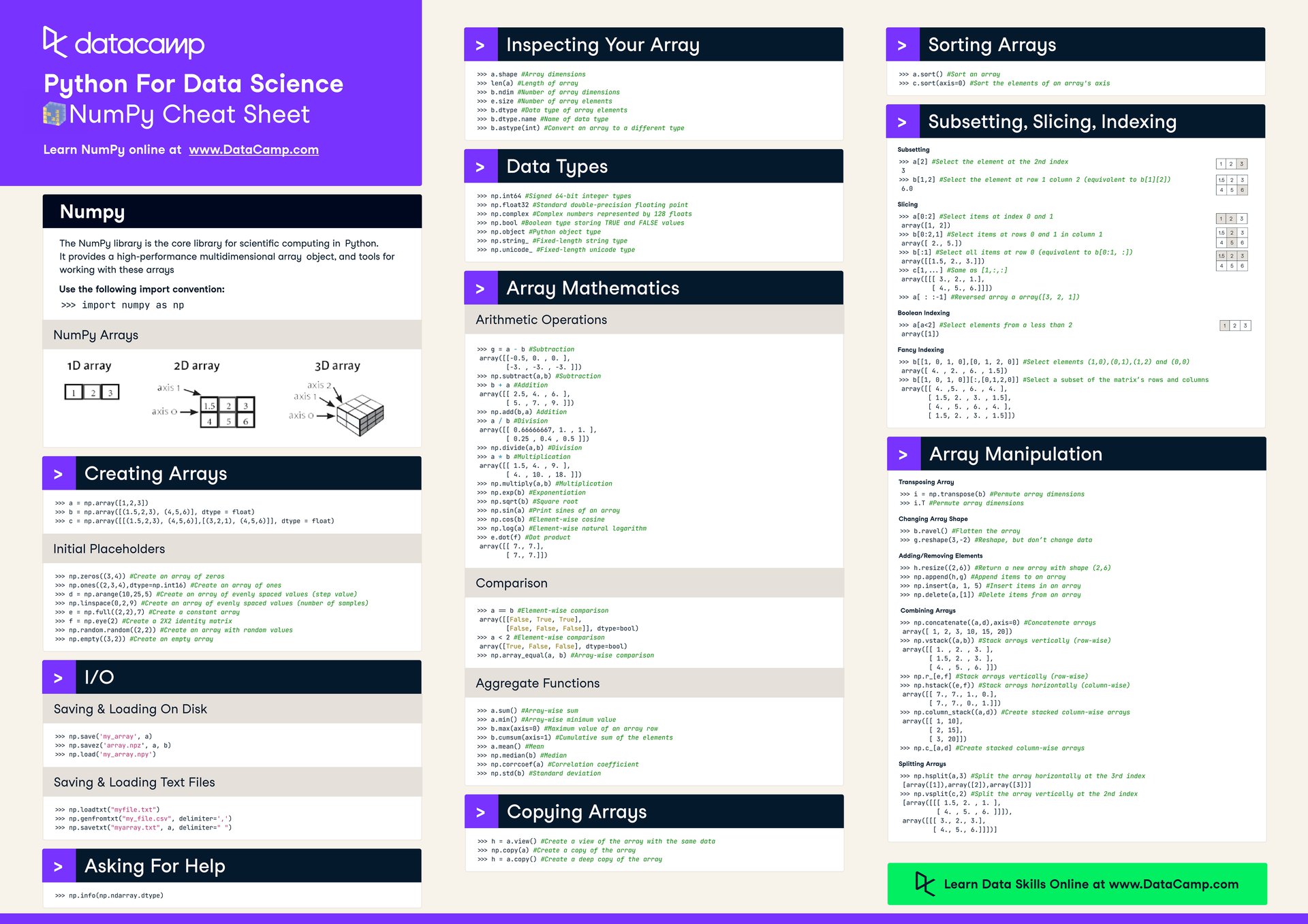
📋 Click to view NumPy Cheat Sheets

Basics
NumPy Architecture
    NumPy Ecosystem
    ┌──────────────────────────────────────────────┐
    │         High-Level Libraries                 │
    │  ┌────────┐ ┌────────┐ ┌────────┐           │
    │  │ Pandas │ │ SciPy  │ │ Scikit │           │
    │  └────┬───┘ └───┬────┘ └───┬────┘           │
    └───────┼─────────┼──────────┼────────────────┘
            │         │          │
    ┌───────▼─────────▼──────────▼────────────────┐
    │           NumPy Core (ndarray)               │
    │  ┌────────────────────────────────────────┐  │
    │  │  Python Interface Layer                │  │
    │  └───────────┬────────────────────────────┘  │
    │              │                                │
    │  ┌───────────▼────────────────────────────┐  │
    │  │  C/Fortran Optimized Routines          │  │
    │  │  (BLAS, LAPACK, etc.)                  │  │
    │  └────────────────────────────────────────┘  │
    └───────────────────────────────────────────────┘
Array Memory Layout
    1D Array: [1, 2, 3, 4]
    ┌───┬───┬───┬───┐
    │ 1 │ 2 │ 3 │ 4 │  Memory: Contiguous block
    └───┴───┴───┴───┘
     ↑
     Base pointer

    2D Array (C-order - Row Major):
    [[1, 2, 3],
     [4, 5, 6]]

    Memory Layout:
    ┌───┬───┬───┬───┬───┬───┐
    │ 1 │ 2 │ 3 │ 4 │ 5 │ 6 │
    └───┴───┴───┴───┴───┴───┘
     Row 0 ────┘   Row 1 ────┘

    2D Array (F-order - Column Major):
    Memory Layout:
    ┌───┬───┬───┬───┬───┬───┐
    │ 1 │ 4 │ 2 │ 5 │ 3 │ 6 │
    └───┴───┴───┴───┴───┴───┘
     Col 0 ─┘   Col 1 ─┘   Col 2 ─┘
In [1]:
Copied!
import numpy as np  # Importing NumPy
np.__version__  # Check version of NumPy
import numpy as np # Importing NumPy np.__version__ # Check version of NumPy
Out[1]:
'1.26.4'
Array Creation
    Creating NumPy Arrays
    ┌─────────────┐
    │   Source    │
    └──────┬──────┘
           │
    ┌──────▼──────────────────────┐
    │                             │
    ▼                             ▼
┌────────────┐            ┌──────────────┐
│ From Data  │            │  Generated   │
└─────┬──────┘            └──────┬───────┘
      │                          │
    ┌─▼────────────┐      ┌──────▼─────────────┐
    │ • Lists      │      │ • zeros/ones/empty │
    │ • Tuples     │      │ • arange/linspace  │
    │ • Buffers    │      │ • random           │
    │ • Files      │      │ • identity         │
    └──────────────┘      └────────────────────┘
From Lists, Tuples, and Buffers
    From Python Collections → NumPy Array

    List:  [1, 2, 3]  ──────┐
                             │
    Tuple: (4, 5, 6)  ───────┼──→  np.array()  ──→  [1 2 3 4 5 6]
                             │
    Buffer: b'data'   ───────┘
In [2]:
Copied!
arr1 = np.array([1, 2, 3])
arr1
arr1 = np.array([1, 2, 3]) arr1
Out[2]:
array([1, 2, 3])
In [3]:
Copied!
arr2 = np.array((1, 2, 3))
arr2
arr2 = np.array((1, 2, 3)) arr2
Out[3]:
array([1, 2, 3])
In [4]:
Copied!
arr3 = np.frombuffer(b'Hello World', dtype='S1')
arr3
arr3 = np.frombuffer(b'Hello World', dtype='S1') arr3
Out[4]:
array([b'H', b'e', b'l', b'l', b'o', b' ', b'W', b'o', b'r', b'l', b'd'],
      dtype='|S1')
Zeros, Ones, and Empty Arrays
    Initialization Arrays

    zeros((2,3))      ones((2,3))       empty((2,3))
    ┌───┬───┬───┐    ┌───┬───┬───┐    ┌───┬───┬───┐
    │ 0 │ 0 │ 0 │    │ 1 │ 1 │ 1 │    │ ? │ ? │ ? │
    ├───┼───┼───┤    ├───┼───┼───┤    ├───┼───┼───┤
    │ 0 │ 0 │ 0 │    │ 1 │ 1 │ 1 │    │ ? │ ? │ ? │
    └───┴───┴───┘    └───┴───┴───┘    └───┴───┴───┘
     All zeros       All ones          Uninitialized
In [5]:
Copied!
arr_zeros = np.zeros((2, 3))  # 2x3 array of zeros
arr_zeros
arr_zeros = np.zeros((2, 3)) # 2x3 array of zeros arr_zeros
Out[5]:
array([[0., 0., 0.],
       [0., 0., 0.]])
In [6]:
Copied!
arr_ones = np.ones((2, 3))  # 2x3 array of ones
arr_ones
arr_ones = np.ones((2, 3)) # 2x3 array of ones arr_ones
Out[6]:
array([[1., 1., 1.],
       [1., 1., 1.]])
In [7]:
Copied!
arr_empty = np.empty((2, 3))  # 2x3 empty array
arr_empty
arr_empty = np.empty((2, 3)) # 2x3 empty array arr_empty
Out[7]:
array([[1., 1., 1.],
       [1., 1., 1.]])
In [ ]:
Copied!
# Create empty array and fill it
arr_empty_filled = np.empty((2, 3))
arr_empty_filled.fill(5)  # Fill with a specific value
arr_empty_filled
# Create empty array and fill it arr_empty_filled = np.empty((2, 3)) arr_empty_filled.fill(5) # Fill with a specific value arr_empty_filled
Ranges and Random Numbers
    Range & Spacing Functions

    arange(0, 10, 2)        linspace(0, 1, 5)
    ┌───────────────┐       ┌───────────────────┐
    │ Start: 0      │       │ Start: 0          │
    │ Stop:  10     │       │ Stop:  1          │
    │ Step:  2      │       │ Count: 5          │
    └───────┬───────┘       └────────┬──────────┘
            │                        │
            ▼                        ▼
      [0, 2, 4, 6, 8]         [0.0, 0.25, 0.5, 0.75, 1.0]
      (excludes stop)         (includes stop)
In [8]:
Copied!
arr_range = np.arange(0, 10, 2)  # Array from 0 to 9 with step 2
arr_range
arr_range = np.arange(0, 10, 2) # Array from 0 to 9 with step 2 arr_range
Out[8]:
array([0, 2, 4, 6, 8])
In [9]:
Copied!
arr_linspace = np.linspace(0, 1, 5)  # 5 equally spaced numbers from 0 to 1
arr_linspace
arr_linspace = np.linspace(0, 1, 5) # 5 equally spaced numbers from 0 to 1 arr_linspace
Out[9]:
array([0. , 0.25, 0.5 , 0.75, 1. ])
In [10]:
Copied!
arr_random = np.random.rand(2, 3)  # 2x3 array with random numbers between 0 and 1
arr_random
arr_random = np.random.rand(2, 3) # 2x3 array with random numbers between 0 and 1 arr_random
Out[10]:
array([[0.78160058, 0.52687888, 0.29604995],
       [0.63947724, 0.99231115, 0.3488577 ]])
In [ ]:
Copied!
# Random integers in a range
arr_randint_range = np.random.randint(10, 20, size=5)  # 5 random integers between 10-19
arr_randint_range
# Random integers in a range arr_randint_range = np.random.randint(10, 20, size=5) # 5 random integers between 10-19 arr_randint_range
Identity and Diagonal Matrices
    Identity Matrix           Diagonal Matrix

    eye(3)                   diag([1, 2, 3])
    ┌───┬───┬───┐            ┌───┬───┬───┐
    │ 1 │ 0 │ 0 │            │ 1 │ 0 │ 0 │
    ├───┼───┼───┤            ├───┼───┼───┤
    │ 0 │ 1 │ 0 │            │ 0 │ 2 │ 0 │
    ├───┼───┼───┤            ├───┼───┼───┤
    │ 0 │ 0 │ 1 │            │ 0 │ 0 │ 3 │
    └───┴───┴───┘            └───┴───┴───┘
In [11]:
Copied!
arr_identity = np.eye(3)  # 3x3 identity matrix
arr_identity
arr_identity = np.eye(3) # 3x3 identity matrix arr_identity
Out[11]:
array([[1., 0., 0.],
       [0., 1., 0.],
       [0., 0., 1.]])
In [12]:
Copied!
arr_diag = np.diag([1, 2, 3])  # Diagonal matrix from a list
arr_diag
arr_diag = np.diag([1, 2, 3]) # Diagonal matrix from a list arr_diag
Out[12]:
array([[1, 0, 0],
       [0, 2, 0],
       [0, 0, 3]])
Structured Arrays
In [13]:
Copied!
dt = np.dtype([('age', np.int32), ('name', np.str_, 10)])
arr_structured = np.array([(21, 'Alice'), (25, 'Bob')], dtype=dt)
arr_structured
dt = np.dtype([('age', np.int32), ('name', np.str_, 10)]) arr_structured = np.array([(21, 'Alice'), (25, 'Bob')], dtype=dt) arr_structured
Out[13]:
array([(21, 'Alice'), (25, 'Bob')],
      dtype=[('age', '<i4'), ('name', '<U10')])
Using np.full and np.tile
In [14]:
Copied!
arr_full = np.full((2, 3), 7)  # Create a 2x3 array filled with the value 7
arr_full
arr_full = np.full((2, 3), 7) # Create a 2x3 array filled with the value 7 arr_full
Out[14]:
array([[7, 7, 7],
       [7, 7, 7]])
In [15]:
Copied!
arr_tile = np.tile([1, 2], (2, 3))  # Repeat [1, 2] in a 2x3 grid
arr_tile
arr_tile = np.tile([1, 2], (2, 3)) # Repeat [1, 2] in a 2x3 grid arr_tile
Out[15]:
array([[1, 2, 1, 2, 1, 2],
       [1, 2, 1, 2, 1, 2]])
Array Inspection
Shape and Size
    Array Properties

    Array: [[1, 2, 3],
            [4, 5, 6]]

    ┌─────────────┐
    │ shape       │──→ (2, 3)     # 2 rows, 3 columns
    ├─────────────┤
    │ size        │──→ 6          # Total elements
    ├─────────────┤
    │ ndim        │──→ 2          # Number of dimensions
    ├─────────────┤
    │ dtype       │──→ int64      # Data type
    ├─────────────┤
    │ itemsize    │──→ 8          # Bytes per element
    ├─────────────┤
    │ nbytes      │──→ 48         # Total bytes (6 * 8)
    └─────────────┘
In [16]:
Copied!
arr1.shape # Dimensions of the array
arr1.shape # Dimensions of the array
Out[16]:
(3,)
In [17]:
Copied!
arr1.size # Total number of elements
arr1.size # Total number of elements
Out[17]:
3
In [18]:
Copied!
arr1.ndim # Number of dimensions
arr1.ndim # Number of dimensions
Out[18]:
1
In [ ]:
Copied!
# Create 2D array for better demonstration
arr_2d = np.array([[1, 2, 3], [4, 5, 6]])
print(f"Shape: {arr_2d.shape}")
print(f"Size: {arr_2d.size}")
print(f"Dimensions: {arr_2d.ndim}")
print(f"Dtype: {arr_2d.dtype}")
arr_2d
# Create 2D array for better demonstration arr_2d = np.array([[1, 2, 3], [4, 5, 6]]) print(f"Shape: {arr_2d.shape}") print(f"Size: {arr_2d.size}") print(f"Dimensions: {arr_2d.ndim}") print(f"Dtype: {arr_2d.dtype}") arr_2d
Data Type
In [19]:
Copied!
arr1.dtype # Data type of elements
arr1.dtype # Data type of elements
Out[19]:
dtype('int64') In [20]:
Copied!
arr1_float = arr1.astype(float)  # Convert to another type
arr1_float
arr1_float = arr1.astype(float) # Convert to another type arr1_float
Out[20]:
array([1., 2., 3.])
Memory Layout
In [21]:
Copied!
arr1.itemsize # Size of one element in bytes
arr1.itemsize # Size of one element in bytes
Out[21]:
8
In [22]:
Copied!
arr1.nbytes # Total memory used by array
arr1.nbytes # Total memory used by array
Out[22]:
24
In [23]:
Copied!
arr1.flags # Memory layout information
arr1.flags # Memory layout information
Out[23]:
  C_CONTIGUOUS : True
  F_CONTIGUOUS : True
  OWNDATA : True
  WRITEABLE : True
  ALIGNED : True
  WRITEBACKIFCOPY : False
Checking for NaN and Inf Values
In [24]:
Copied!
arr_nan_inf = np.array([1, 2, np.nan, np.inf])
np.isnan(arr_nan_inf), np.isinf(arr_nan_inf), np.isfinite(arr_nan_inf)
arr_nan_inf = np.array([1, 2, np.nan, np.inf]) np.isnan(arr_nan_inf), np.isinf(arr_nan_inf), np.isfinite(arr_nan_inf)
Out[24]:
(array([False, False,  True, False]),
 array([False, False, False,  True]),
 array([ True,  True, False, False]))
Array Mathematics
Basic Operations
    Element-wise Operations (Broadcasting)

    Array:  [1, 2, 3]
    Scalar: 2

    ┌───┬───┬───┐        ┌───┬───┬───┐
    │ 1 │ 2 │ 3 │   +2   │ 3 │ 4 │ 5 │
    └───┴───┴───┘   ══→  └───┴───┴───┘

    ┌───┬───┬───┐        ┌───┬───┬───┐
    │ 1 │ 2 │ 3 │   *2   │ 2 │ 4 │ 6 │
    └───┴───┴───┘   ══→  └───┴───┴───┘

    Array-Array Operations:
    [1, 2, 3] + [4, 5, 6] = [5, 7, 9]
In [25]:
Copied!
arr_add = arr1 + 1  # Add 1 to each element
arr_add
arr_add = arr1 + 1 # Add 1 to each element arr_add
Out[25]:
array([2, 3, 4])
In [26]:
Copied!
arr_mul = arr1 * 2  # Multiply each element by 2
arr_mul
arr_mul = arr1 * 2 # Multiply each element by 2 arr_mul
Out[26]:
array([2, 4, 6])
In [27]:
Copied!
arr_sum = np.add(arr1, arr2)  # Add arrays element-wise
arr_sum
arr_sum = np.add(arr1, arr2) # Add arrays element-wise arr_sum
Out[27]:
array([2, 4, 6])
In [28]:
Copied!
arr_diff = np.subtract(arr1, arr2)  # Subtract arrays element-wise
arr_diff
arr_diff = np.subtract(arr1, arr2) # Subtract arrays element-wise arr_diff
Out[28]:
array([0, 0, 0])
In [ ]:
Copied!
# More operations
arr_prod_elem = np.multiply(arr1, arr2)  # Element-wise multiplication
arr_div = np.divide(arr1, arr2)  # Element-wise division
arr_power = np.power(arr1, 2)  # Square each element
print(f"Multiply: {arr_prod_elem}")
print(f"Divide: {arr_div}")
print(f"Power: {arr_power}")
# More operations arr_prod_elem = np.multiply(arr1, arr2) # Element-wise multiplication arr_div = np.divide(arr1, arr2) # Element-wise division arr_power = np.power(arr1, 2) # Square each element print(f"Multiply: {arr_prod_elem}") print(f"Divide: {arr_div}") print(f"Power: {arr_power}")
Aggregate Functions
    Aggregate Functions Flow

    Array: [1, 2, 3, 4, 5]
           │
    ┌──────┴───────┬──────────┬──────────┐
    │              │          │          │
    ▼              ▼          ▼          ▼
  sum()        mean()      max()      min()
    │              │          │          │
    ▼              ▼          ▼          ▼
    15            3.0         5          1

    Axis-wise Operations (2D):
    [[1, 2],
     [3, 4]]

    axis=0 (↓)    axis=1 (→)    axis=None (all)
    [4, 6]        [3, 7]        15
In [29]:
Copied!
arr_sum_total = np.sum(arr1)  # Sum of all elements
arr_sum_total
arr_sum_total = np.sum(arr1) # Sum of all elements arr_sum_total
Out[29]:
6
In [30]:
Copied!
arr_mean = np.mean(arr1)  # Mean of elements
arr_mean
arr_mean = np.mean(arr1) # Mean of elements arr_mean
Out[30]:
2.0
In [31]:
Copied!
arr_max = np.max(arr1)  # Maximum value
arr_max
arr_max = np.max(arr1) # Maximum value arr_max
Out[31]:
3
In [32]:
Copied!
arr_min = np.min(arr1)  # Minimum value
arr_min
arr_min = np.min(arr1) # Minimum value arr_min
Out[32]:
1
In [33]:
Copied!
arr_prod = np.prod(arr1)  # Product of elements
arr_prod
arr_prod = np.prod(arr1) # Product of elements arr_prod
Out[33]:
6
In [34]:
Copied!
arr_cumsum = np.cumsum(arr1)  # Cumulative sum of elements
arr_cumsum
arr_cumsum = np.cumsum(arr1) # Cumulative sum of elements arr_cumsum
Out[34]:
array([1, 3, 6])
In [35]:
Copied!
arr_cumprod = np.cumprod(arr1)  # Cumulative product of elements
arr_cumprod
arr_cumprod = np.cumprod(arr1) # Cumulative product of elements arr_cumprod
Out[35]:
array([1, 2, 6])
In [ ]:
Copied!
# Axis-wise aggregations
arr_2d_demo = np.array([[1, 2, 3], [4, 5, 6]])
print(f"Sum all: {np.sum(arr_2d_demo)}")
print(f"Sum axis 0 (columns): {np.sum(arr_2d_demo, axis=0)}")
print(f"Sum axis 1 (rows): {np.sum(arr_2d_demo, axis=1)}")
print(f"Mean axis 0: {np.mean(arr_2d_demo, axis=0)}")
print(f"Max axis 1: {np.max(arr_2d_demo, axis=1)}")
# Axis-wise aggregations arr_2d_demo = np.array([[1, 2, 3], [4, 5, 6]]) print(f"Sum all: {np.sum(arr_2d_demo)}") print(f"Sum axis 0 (columns): {np.sum(arr_2d_demo, axis=0)}") print(f"Sum axis 1 (rows): {np.sum(arr_2d_demo, axis=1)}") print(f"Mean axis 0: {np.mean(arr_2d_demo, axis=0)}") print(f"Max axis 1: {np.max(arr_2d_demo, axis=1)}")
Exponentials and Logarithms
In [36]:
Copied!
arr_exp = np.exp(arr1)  # Exponential of each element
arr_exp
arr_exp = np.exp(arr1) # Exponential of each element arr_exp
Out[36]:
array([ 2.71828183, 7.3890561 , 20.08553692])
In [37]:
Copied!
arr_log = np.log(arr1)  # Natural logarithm
arr_log
arr_log = np.log(arr1) # Natural logarithm arr_log
Out[37]:
array([0. , 0.69314718, 1.09861229])
In [38]:
Copied!
arr_log10 = np.log10(arr1)  # Base-10 logarithm
arr_log10
arr_log10 = np.log10(arr1) # Base-10 logarithm arr_log10
Out[38]:
array([0. , 0.30103 , 0.47712125])
In [39]:
Copied!
arr_expm1 = np.expm1(arr1)  # Compute exp(x) - 1
arr_expm1
arr_expm1 = np.expm1(arr1) # Compute exp(x) - 1 arr_expm1
Out[39]:
array([ 1.71828183, 6.3890561 , 19.08553692])
Trigonometric Functions
In [40]:
Copied!
arr_sin = np.sin(arr1)  # Sine of each element
arr_sin
arr_sin = np.sin(arr1) # Sine of each element arr_sin
Out[40]:
array([0.84147098, 0.90929743, 0.14112001])
In [41]:
Copied!
arr_cos = np.cos(arr1)  # Cosine of each element
arr_cos
arr_cos = np.cos(arr1) # Cosine of each element arr_cos
Out[41]:
array([ 0.54030231, -0.41614684, -0.9899925 ])
In [42]:
Copied!
arr_tan = np.tan(arr1)  # Tangent of each element
arr_tan
arr_tan = np.tan(arr1) # Tangent of each element arr_tan
Out[42]:
array([ 1.55740772, -2.18503986, -0.14254654])
In [43]:
Copied!
arr_arcsin = np.arcsin(arr1 / 10)  # Inverse sine
arr_arcsin
arr_arcsin = np.arcsin(arr1 / 10) # Inverse sine arr_arcsin
Out[43]:
array([0.10016742, 0.20135792, 0.30469265])
In [44]:
Copied!
arr_arccos = np.arccos(arr1 / 10)  # Inverse cosine
arr_arccos
arr_arccos = np.arccos(arr1 / 10) # Inverse cosine arr_arccos
Out[44]:
array([1.47062891, 1.36943841, 1.26610367])
In [45]:
Copied!
arr_arctan = np.arctan(arr1 / 10)  # Inverse tangent
arr_arctan
arr_arctan = np.arctan(arr1 / 10) # Inverse tangent arr_arctan
Out[45]:
array([0.09966865, 0.19739556, 0.29145679])
Rounding and Precision Control
In [46]:
Copied!
arr_round = np.round(arr1_float, decimals=2)  # Round to 2 decimal places
arr_round
arr_round = np.round(arr1_float, decimals=2) # Round to 2 decimal places arr_round
Out[46]:
array([1., 2., 3.])
In [47]:
Copied!
arr_floor = np.floor(arr1_float)  # Floor operation
arr_floor
arr_floor = np.floor(arr1_float) # Floor operation arr_floor
Out[47]:
array([1., 2., 3.])
In [48]:
Copied!
arr_ceil = np.ceil(arr1_float)  # Ceiling operation
arr_ceil
arr_ceil = np.ceil(arr1_float) # Ceiling operation arr_ceil
Out[48]:
array([1., 2., 3.])
In [49]:
Copied!
arr_trunc = np.trunc(arr1_float)  # Truncate elements to integers
arr_trunc
arr_trunc = np.trunc(arr1_float) # Truncate elements to integers arr_trunc
Out[49]:
array([1., 2., 3.])
Array Manipulation
Reshaping
    Array Reshaping & Transposing

    Original (1D):          Reshaped (2D):
    [1, 2, 3, 4, 5, 6]  ──→  [[1, 2, 3],
     6 elements               [4, 5, 6]]
                             2×3 = 6 ✓

    Transpose:
    [[1, 2, 3],         [[1, 4],
     [4, 5, 6]]    ──→   [2, 5],
     (2, 3)              [3, 6]]
                         (3, 2)

    Flatten:
    [[1, 2],
     [3, 4]]        ──→  [1, 2, 3, 4]
     (2, 2)              (4,)
In [50]:
Copied!
arr_reshaped = arr1.reshape((3, 1))  # Reshape to 3x1 array
arr_reshaped
arr_reshaped = arr1.reshape((3, 1)) # Reshape to 3x1 array arr_reshaped
Out[50]:
array([[1],
       [2],
       [3]])
In [51]:
Copied!
arr_flattened = arr1.flatten()  # Flatten the array to 1D
arr_flattened
arr_flattened = arr1.flatten() # Flatten the array to 1D arr_flattened
Out[51]:
array([1, 2, 3])
In [52]:
Copied!
arr_raveled = np.ravel(arr1)  # Return a flattened array
arr_raveled
arr_raveled = np.ravel(arr1) # Return a flattened array arr_raveled
Out[52]:
array([1, 2, 3])
In [ ]:
Copied!
# Reshape with -1 (auto-calculate dimension)
arr_auto_reshape = np.arange(12).reshape(3, -1)  # Auto calculates 4 columns
print(f"Auto reshaped to shape: {arr_auto_reshape.shape}")
arr_auto_reshape
# Reshape with -1 (auto-calculate dimension) arr_auto_reshape = np.arange(12).reshape(3, -1) # Auto calculates 4 columns print(f"Auto reshaped to shape: {arr_auto_reshape.shape}") arr_auto_reshape
Transposing
In [53]:
Copied!
arr_T = arr1.reshape((1, 3)).T  # Transpose of the array
arr_T
arr_T = arr1.reshape((1, 3)).T # Transpose of the array arr_T
Out[53]:
array([[1],
       [2],
       [3]])
In [54]:
Copied!
arr_custom_T = np.transpose(arr1.reshape((3, 1)), (1, 0))  # Custom transpose
arr_custom_T
arr_custom_T = np.transpose(arr1.reshape((3, 1)), (1, 0)) # Custom transpose arr_custom_T
Out[54]:
array([[1, 2, 3]])
Joining and Splitting Arrays
    Concatenating Arrays

    Horizontal Stack (hstack):          Vertical Stack (vstack):
    [1, 2] + [3, 4] ──→ [1, 2, 3, 4]   [1, 2]  ──→  [[1, 2],
                                        [3, 4]        [3, 4]]

    Concatenate along axis:

    axis=0 (vertical):      axis=1 (horizontal):
    [[1, 2],                [[1, 2],
     [3, 4]]    +            [3, 4]]    +
    [[5, 6]]     ─→          [[7, 8]]    ─→
    [[1, 2],                [[1, 2, 7, 8],
     [3, 4],                 [3, 4, ?  ? ]]  ← Error!
     [5, 6]]                (shape mismatch)
In [55]:
Copied!
arr_concat = np.concatenate((arr1, arr2))  # Join arrays
arr_concat
arr_concat = np.concatenate((arr1, arr2)) # Join arrays arr_concat
Out[55]:
array([1, 2, 3, 1, 2, 3])
In [56]:
Copied!
arr_hstack = np.hstack((arr1.reshape((3, 1)), arr2.reshape((3, 1))))  # Horizontal stack
arr_hstack
arr_hstack = np.hstack((arr1.reshape((3, 1)), arr2.reshape((3, 1)))) # Horizontal stack arr_hstack
Out[56]:
array([[1, 1],
       [2, 2],
       [3, 3]])
In [57]:
Copied!
arr_vstack = np.vstack((arr1, arr2))  # Vertical stack
arr_vstack
arr_vstack = np.vstack((arr1, arr2)) # Vertical stack arr_vstack
Out[57]:
array([[1, 2, 3],
       [1, 2, 3]])
In [58]:
Copied!
arr_split = np.split(arr_concat, 3)  # Split into 3 equal parts
arr_split
arr_split = np.split(arr_concat, 3) # Split into 3 equal parts arr_split
Out[58]:
[array([1, 2]), array([3, 1]), array([2, 3])]
In [59]:
Copied!
arr_hsplit = np.hsplit(arr_hstack, 2)  # Split horizontally
arr_hsplit
arr_hsplit = np.hsplit(arr_hstack, 2) # Split horizontally arr_hsplit
Out[59]:
[array([[1],
        [2],
        [3]]),
 array([[1],
        [2],
        [3]])]
In [60]:
Copied!
arr_vsplit = np.vsplit(arr_vstack, 2)  # Split vertically
arr_vsplit
arr_vsplit = np.vsplit(arr_vstack, 2) # Split vertically arr_vsplit
Out[60]:
[array([[1, 2, 3]]), array([[1, 2, 3]])]
In [ ]:
Copied!
# Column stack and row stack
arr_col = np.array([1, 2, 3])
arr_col2 = np.array([4, 5, 6])
arr_column_stack = np.column_stack((arr_col, arr_col2))  # Stack as columns
arr_row_stack = np.row_stack((arr_col, arr_col2))  # Stack as rows
print("Column stack:")
print(arr_column_stack)
print("\nRow stack:")
print(arr_row_stack)
# Column stack and row stack arr_col = np.array([1, 2, 3]) arr_col2 = np.array([4, 5, 6]) arr_column_stack = np.column_stack((arr_col, arr_col2)) # Stack as columns arr_row_stack = np.row_stack((arr_col, arr_col2)) # Stack as rows print("Column stack:") print(arr_column_stack) print("\nRow stack:") print(arr_row_stack)
Changing Dimensions
In [61]:
Copied!
arr_expanded = np.expand_dims(arr1, axis=0)  # Expand dimensions
arr_expanded
arr_expanded = np.expand_dims(arr1, axis=0) # Expand dimensions arr_expanded
Out[61]:
array([[1, 2, 3]])
In [62]:
Copied!
arr_squeezed = np.squeeze(arr_expanded)  # Remove single-dimensional entries
arr_squeezed
arr_squeezed = np.squeeze(arr_expanded) # Remove single-dimensional entries arr_squeezed
Out[62]:
array([1, 2, 3])
Array Repetition
In [63]:
Copied!
arr_tiled = np.tile(arr1, (2, 3))  # Repeat array
arr_tiled
arr_tiled = np.tile(arr1, (2, 3)) # Repeat array arr_tiled
Out[63]:
array([[1, 2, 3, 1, 2, 3, 1, 2, 3],
       [1, 2, 3, 1, 2, 3, 1, 2, 3]])
In [64]:
Copied!
arr_repeated = np.repeat(arr1, 3)  # Repeat elements of an array
arr_repeated
arr_repeated = np.repeat(arr1, 3) # Repeat elements of an array arr_repeated
Out[64]:
array([1, 1, 1, 2, 2, 2, 3, 3, 3])
Rotating and Flipping Arrays
In [65]:
Copied!
arr_rot90 = np.rot90(arr1.reshape((3, 1)))  # Rotate array by 90 degrees
arr_rot90
arr_rot90 = np.rot90(arr1.reshape((3, 1))) # Rotate array by 90 degrees arr_rot90
Out[65]:
array([[1, 2, 3]])
In [66]:
Copied!
arr_fliplr = np.fliplr(arr1.reshape((3, 1)))  # Flip array left to right
arr_fliplr
arr_fliplr = np.fliplr(arr1.reshape((3, 1))) # Flip array left to right arr_fliplr
Out[66]:
array([[1],
       [2],
       [3]])
In [67]:
Copied!
arr_flipud = np.flipud(arr1.reshape((3, 1)))  # Flip array upside down
arr_flipud
arr_flipud = np.flipud(arr1.reshape((3, 1))) # Flip array upside down arr_flipud
Out[67]:
array([[3],
       [2],
       [1]])
Linear Algebra
Dot Product and Matrix Multiplication
    Matrix Operations

    Dot Product (1D):
    [1, 2, 3] · [4, 5, 6] = 1×4 + 2×5 + 3×6 = 32

    Matrix Multiplication:
    [[a, b],     [[e, f],     [[ae+bg, af+bh],
     [c, d]]  @   [g, h]]  =   [ce+dg, cf+dh]]
     (2×2)        (2×2)         (2×2)

    Key: (m×n) @ (n×p) = (m×p)
         ────     ─
         Must match!

    Linear System Ax = b:
    ┌──────────┐     ┌───┐     ┌───┐
    │ 3   1    │  @  │ x │  =  │ 9 │
    │ 1   2    │     │ y │     │ 8 │
    └──────────┘     └───┘     └───┘
         A            x          b
                      ↓
              solve(A, b) → x
In [68]:
Copied!
arr_dot = np.dot(arr1, arr2)  # Dot product
arr_dot
arr_dot = np.dot(arr1, arr2) # Dot product arr_dot
Out[68]:
14
In [69]:
Copied!
arr_matmul = np.matmul(arr1.reshape((3, 1)), arr2.reshape((1, 3)))  # Matrix multiplication
arr_matmul
arr_matmul = np.matmul(arr1.reshape((3, 1)), arr2.reshape((1, 3))) # Matrix multiplication arr_matmul
Out[69]:
array([[1, 2, 3],
       [2, 4, 6],
       [3, 6, 9]])
In [70]:
Copied!
arr_matmul_op = arr1.reshape((3, 1)) @ arr2.reshape((1, 3))  # Matrix multiplication using @
arr_matmul_op
arr_matmul_op = arr1.reshape((3, 1)) @ arr2.reshape((1, 3)) # Matrix multiplication using @ arr_matmul_op
Out[70]:
array([[1, 2, 3],
       [2, 4, 6],
       [3, 6, 9]])
In [ ]:
Copied!
# Inner and outer products
arr_inner = np.inner(arr1, arr2)  # Inner product (same as dot for 1D)
arr_outer_demo = np.outer(arr1, arr2)  # Outer product
print(f"Inner product: {arr_inner}")
print(f"Outer product:\n{arr_outer_demo}")
# Inner and outer products arr_inner = np.inner(arr1, arr2) # Inner product (same as dot for 1D) arr_outer_demo = np.outer(arr1, arr2) # Outer product print(f"Inner product: {arr_inner}") print(f"Outer product:\n{arr_outer_demo}")
Solving Linear Equations
In [71]:
Copied!
A = np.array([[3, 1], [1, 2]])
b = np.array([9, 8])
x = np.linalg.solve(A, b)  # Solve linear equations Ax = b
x
A = np.array([[3, 1], [1, 2]]) b = np.array([9, 8]) x = np.linalg.solve(A, b) # Solve linear equations Ax = b x
Out[71]:
array([2., 3.])
Eigenvalues and Eigenvectors
In [72]:
Copied!
arr_eigvals, arr_eigvecs = np.linalg.eig(A)  # Eigenvalues and eigenvectors
arr_eigvals, arr_eigvecs
arr_eigvals, arr_eigvecs = np.linalg.eig(A) # Eigenvalues and eigenvectors arr_eigvals, arr_eigvecs
Out[72]:
(array([3.61803399, 1.38196601]),
 array([[ 0.85065081, -0.52573111],
        [ 0.52573111,  0.85065081]]))
Inverse and Determinant
    Matrix Decompositions

    Eigendecomposition:
    A = V Λ V⁻¹
    │   │ │  └─ Eigenvectors (inverse)
    │   │ └──── Eigenvalues (diagonal matrix)
    │   └────── Eigenvectors
    └────────── Original matrix

    SVD (Singular Value Decomposition):
    A = U Σ Vᵀ
    │   │ │ └─ Right singular vectors
    │   │ └─── Singular values (diagonal)
    │   └───── Left singular vectors
    └───────── Original matrix

    Applications:
    • Eigenvalues  → Stability analysis
    • Inverse      → Solving linear systems
    • Determinant  → Matrix properties
    • SVD          → Dimensionality reduction
In [73]:
Copied!
arr_inv = np.linalg.inv(A)  # Inverse of a matrix
arr_inv
arr_inv = np.linalg.inv(A) # Inverse of a matrix arr_inv
Out[73]:
array([[ 0.4, -0.2],
       [-0.2,  0.6]])
In [74]:
Copied!
arr_det = np.linalg.det(A)  # Determinant of a matrix
arr_det
arr_det = np.linalg.det(A) # Determinant of a matrix arr_det
Out[74]:
5.000000000000001
In [ ]:
Copied!
# Matrix rank and trace
arr_rank_demo = np.linalg.matrix_rank(A)  # Number of linearly independent rows/cols
arr_trace_demo = np.trace(A)  # Sum of diagonal elements
print(f"Matrix rank: {arr_rank_demo}")
print(f"Matrix trace: {arr_trace_demo}")
print(f"Determinant: {arr_det}")
# Matrix rank and trace arr_rank_demo = np.linalg.matrix_rank(A) # Number of linearly independent rows/cols arr_trace_demo = np.trace(A) # Sum of diagonal elements print(f"Matrix rank: {arr_rank_demo}") print(f"Matrix trace: {arr_trace_demo}") print(f"Determinant: {arr_det}")
Singular Value Decomposition (SVD)
In [75]:
Copied!
U, S, V = np.linalg.svd(A)  # Singular Value Decomposition
U, S, V
U, S, V = np.linalg.svd(A) # Singular Value Decomposition U, S, V
Out[75]:
(array([[-0.85065081, -0.52573111],
        [-0.52573111,  0.85065081]]),
 array([3.61803399, 1.38196601]),
 array([[-0.85065081, -0.52573111],
        [-0.52573111,  0.85065081]]))
Norms and Condition Numbers
In [76]:
Copied!
arr_norm = np.linalg.norm(arr1)  # Compute matrix or vector norm
arr_norm
arr_norm = np.linalg.norm(arr1) # Compute matrix or vector norm arr_norm
Out[76]:
3.7416573867739413
In [77]:
Copied!
arr_cond = np.linalg.cond(A)  # Compute the condition number of a matrix
arr_cond
arr_cond = np.linalg.cond(A) # Compute the condition number of a matrix arr_cond
Out[77]:
2.618033988749896
Statistics
Descriptive Statistics
    Statistical Measures

    Dataset: [1, 2, 3, 4, 5]

    Central Tendency:          Dispersion:
    ┌──────────┐              ┌───────────┐
    │  Mean    │──→ 3.0       │ Variance  │──→ 2.0
    │  Median  │──→ 3.0       │  Std Dev  │──→ 1.41
    │  Mode    │──→ (none)    │   Range   │──→ 4
    └──────────┘              └───────────┘

    Percentiles:

    [1, 2, 3, 4, 5, 6, 7, 8, 9, 10]
     ↑           ↑              ↑
    min        50th           max
    (0%)      (median)       (100%)

    Box Plot Visualization:

         │
      10 ├───┐  ← Q3 (75%)
         │   │
       5 ├───┤  ← Median (50%)
         │   │
       2 ├───┘  ← Q1 (25%)
         │
In [78]:
Copied!
arr_mean = np.mean(arr1)  # Mean
arr_mean
arr_mean = np.mean(arr1) # Mean arr_mean
Out[78]:
2.0
In [79]:
Copied!
arr_median = np.median(arr1)  # Median
arr_median
arr_median = np.median(arr1) # Median arr_median
Out[79]:
2.0
In [80]:
Copied!
arr_var = np.var(arr1)  # Variance
arr_var
arr_var = np.var(arr1) # Variance arr_var
Out[80]:
0.6666666666666666
In [81]:
Copied!
arr_std = np.std(arr1)  # Standard deviation
arr_std
arr_std = np.std(arr1) # Standard deviation arr_std
Out[81]:
0.816496580927726
In [ ]:
Copied!
# Comprehensive statistics example
data_stats = np.array([12, 15, 17, 18, 20, 22, 24, 25, 28, 30])
print(f"Data: {data_stats}")
print(f"\nCentral Tendency:")
print(f"  Mean: {np.mean(data_stats):.2f}")
print(f"  Median: {np.median(data_stats):.2f}")
print(f"\nDispersion:")
print(f"  Variance: {np.var(data_stats):.2f}")
print(f"  Std Dev: {np.std(data_stats):.2f}")
print(f"  Min: {np.min(data_stats)}, Max: {np.max(data_stats)}")
print(f"  Range: {np.ptp(data_stats)}")  # Peak to peak (range)
print(f"\nPercentiles:")
print(f"  25th: {np.percentile(data_stats, 25):.2f}")
print(f"  50th: {np.percentile(data_stats, 50):.2f}")
print(f"  75th: {np.percentile(data_stats, 75):.2f}")
# Comprehensive statistics example data_stats = np.array([12, 15, 17, 18, 20, 22, 24, 25, 28, 30]) print(f"Data: {data_stats}") print(f"\nCentral Tendency:") print(f" Mean: {np.mean(data_stats):.2f}") print(f" Median: {np.median(data_stats):.2f}") print(f"\nDispersion:") print(f" Variance: {np.var(data_stats):.2f}") print(f" Std Dev: {np.std(data_stats):.2f}") print(f" Min: {np.min(data_stats)}, Max: {np.max(data_stats)}") print(f" Range: {np.ptp(data_stats)}") # Peak to peak (range) print(f"\nPercentiles:") print(f" 25th: {np.percentile(data_stats, 25):.2f}") print(f" 50th: {np.percentile(data_stats, 50):.2f}") print(f" 75th: {np.percentile(data_stats, 75):.2f}")
Percentiles
In [82]:
Copied!
arr_percentile = np.percentile(arr1, 50)  # 50th percentile (median)
arr_percentile
arr_percentile = np.percentile(arr1, 50) # 50th percentile (median) arr_percentile
Out[82]:
2.0
Correlation and Covariance
In [83]:
Copied!
arr_corr = np.corrcoef(arr1, arr2)  # Correlation coefficient
arr_corr
arr_corr = np.corrcoef(arr1, arr2) # Correlation coefficient arr_corr
Out[83]:
array([[1., 1.],
       [1., 1.]])
In [84]:
Copied!
arr_cov = np.cov(arr1, arr2)  # Covariance
arr_cov
arr_cov = np.cov(arr1, arr2) # Covariance arr_cov
Out[84]:
array([[1., 1.],
       [1., 1.]])
Histogram
In [85]:
Copied!
arr_hist, arr_bins = np.histogram(arr1, bins=3)  # Histogram of an array
arr_hist, arr_bins
arr_hist, arr_bins = np.histogram(arr1, bins=3) # Histogram of an array arr_hist, arr_bins
Out[85]:
(array([1, 1, 1]), array([1. , 1.66666667, 2.33333333, 3. ]))
Binned Statistics
In [86]:
Copied!
from scipy import stats
arr_binned_statistic = stats.binned_statistic(arr1, arr1, statistic='mean', bins=3)  # Compute binned statistics
arr_binned_statistic.statistic
from scipy import stats arr_binned_statistic = stats.binned_statistic(arr1, arr1, statistic='mean', bins=3) # Compute binned statistics arr_binned_statistic.statistic
Out[86]:
array([1., 2., 3.])
Broadcasting
Basic Broadcasting
    Broadcasting Rules

    Rule 1: If arrays have different dimensions,
            prepend 1s to the shape of the smaller array

    Rule 2: Arrays are compatible if dimensions are
            either equal or one of them is 1

    Example 1: Valid Broadcasting
    ┌─────────────┐     ┌─────┐
    │ (3, 4)      │  +  │ (4,)│  → (3, 4) + (1, 4) ✓
    └─────────────┘     └─────┘
    [[a, b, c, d],      [x, y, z, w]
     [e, f, g, h],   +   (broadcast)
     [i, j, k, l]]

    Example 2: Invalid Broadcasting
    (3, 4) + (3,) → (3, 4) + (1, 3) ✗
    ────       ─
    Mismatch!

    Example 3: 2D Broadcasting
    (3, 1)   +   (1, 4)   →   (3, 4)
    [[a],        [[w, x, y, z]]
     [b],    +   (broadcast both)
     [c]]
In [87]:
Copied!
arr_broadcast_add = arr1 + 5  # Add 5 to all elements
arr_broadcast_add
arr_broadcast_add = arr1 + 5 # Add 5 to all elements arr_broadcast_add
Out[87]:
array([6, 7, 8])
In [88]:
Copied!
arr_broadcast_array = arr1 + np.array([1, 2, 3])  # Add array [1, 2, 3] to each row
arr_broadcast_array
arr_broadcast_array = arr1 + np.array([1, 2, 3]) # Add array [1, 2, 3] to each row arr_broadcast_array
Out[88]:
array([2, 4, 6])
Advanced Broadcasting
In [89]:
Copied!
arr_broadcast_mult = arr1 * np.array([1, 2, 3])  # Element-wise multiplication with broadcasting
arr_broadcast_mult
arr_broadcast_mult = arr1 * np.array([1, 2, 3]) # Element-wise multiplication with broadcasting arr_broadcast_mult
Out[89]:
array([1, 4, 9])
In [90]:
Copied!
arr_broadcast_expand = np.expand_dims(arr1, axis=0) + arr1  # Broadcasting with dimension expansion
arr_broadcast_expand
arr_broadcast_expand = np.expand_dims(arr1, axis=0) + arr1 # Broadcasting with dimension expansion arr_broadcast_expand
Out[90]:
array([[2, 4, 6]])
In [ ]:
Copied!
# 2D broadcasting example
arr_a = np.array([[1], [2], [3]])  # Shape (3, 1)
arr_b = np.array([10, 20, 30])      # Shape (3,) → (1, 3)
arr_broadcast_2d = arr_a + arr_b    # Result shape (3, 3)
print(f"Shape a: {arr_a.shape}, Shape b: {arr_b.shape}")
print(f"Result shape: {arr_broadcast_2d.shape}")
print(arr_broadcast_2d)
# 2D broadcasting example arr_a = np.array([[1], [2], [3]]) # Shape (3, 1) arr_b = np.array([10, 20, 30]) # Shape (3,) → (1, 3) arr_broadcast_2d = arr_a + arr_b # Result shape (3, 3) print(f"Shape a: {arr_a.shape}, Shape b: {arr_b.shape}") print(f"Result shape: {arr_broadcast_2d.shape}") print(arr_broadcast_2d)
Indexing and Slicing
Basic Indexing
    Indexing & Slicing

    1D Array: [0, 1, 2, 3, 4]
              ↑     ↑     ↑
    Index:    0     2     4
    Negative: -5   -3    -1

    Slicing: array[start:stop:step]

    [0, 1, 2, 3, 4]
     ↓  ↓  ↓  ↓  ↓
    [0:5:1]  → [0, 1, 2, 3, 4]  (all)
    [1:4:1]  → [1, 2, 3]         (middle)
    [::2]    → [0, 2, 4]         (every 2nd)
    [::-1]   → [4, 3, 2, 1, 0]  (reverse)

    2D Array: [[1, 2, 3],
               [4, 5, 6]]

    arr[0, :]    → [1, 2, 3]     (first row)
    arr[:, 0]    → [1, 4]         (first column)
    arr[0, 1]    → 2              (element)
    arr[:, 1:3]  → [[2, 3],       (columns 1-2)
                    [5, 6]]
In [91]:
Copied!
first_element = arr1[0]  # First element
first_element
first_element = arr1[0] # First element first_element
Out[91]:
1
In [92]:
Copied!
last_element = arr1[-1]  # Last element
last_element
last_element = arr1[-1] # Last element last_element
Out[92]:
3
In [93]:
Copied!
element_0_2 = arr1[0]  # First element
third_element = arr1[2]  # Third element
first_element, third_element
element_0_2 = arr1[0] # First element third_element = arr1[2] # Third element first_element, third_element
Out[93]:
(1, 3)
Slicing
In [94]:
Copied!
arr_slice_1_3 = arr1[1:3]  # Elements from index 1 to 2
arr_slice_1_3
arr_slice_1_3 = arr1[1:3] # Elements from index 1 to 2 arr_slice_1_3
Out[94]:
array([2, 3])
In [95]:
Copied!
arr_slice_all = arr1[:]  # All elements
arr_slice_all
arr_slice_all = arr1[:] # All elements arr_slice_all
Out[95]:
array([1, 2, 3])
In [96]:
Copied!
arr_slice_skip = arr1[::2]  # Every other element
arr_slice_skip
arr_slice_skip = arr1[::2] # Every other element arr_slice_skip
Out[96]:
array([1, 3])
In [ ]:
Copied!
# 2D indexing examples
arr_2d_idx = np.array([[1, 2, 3, 4], [5, 6, 7, 8], [9, 10, 11, 12]])
print(f"First row: {arr_2d_idx[0, :]}")
print(f"First column: {arr_2d_idx[:, 0]}")
print(f"Last element: {arr_2d_idx[-1, -1]}")
print(f"Middle 2x2:\n{arr_2d_idx[0:2, 1:3]}")
# 2D indexing examples arr_2d_idx = np.array([[1, 2, 3, 4], [5, 6, 7, 8], [9, 10, 11, 12]]) print(f"First row: {arr_2d_idx[0, :]}") print(f"First column: {arr_2d_idx[:, 0]}") print(f"Last element: {arr_2d_idx[-1, -1]}") print(f"Middle 2x2:\n{arr_2d_idx[0:2, 1:3]}")
Fancy Indexing
    Advanced Indexing Techniques

    1. Fancy Indexing (Integer Arrays):
    arr = [10, 20, 30, 40, 50]
          0   1   2   3   4  (indices)

    arr[[0, 2, 4]] → [10, 30, 50]
    arr[[4, 0, 2]] → [50, 10, 30] (order matters!)

    2. Boolean Indexing:
    arr > 25 → [F, F, T, T, T]
    arr[arr > 25] → [30, 40, 50]

    3. Multi-dimensional Fancy Indexing:
    arr_2d = [[1, 2],
              [3, 4]]

    rows = [0, 1]
    cols = [1, 0]
    arr_2d[rows, cols] → [2, 3]
                          ↑  ↑
                        (0,1) (1,0)

    4. Combining Methods:
    mask = arr > 25
    indices = np.where(mask)[0]
    result = arr[indices]
In [97]:
Copied!
arr_fancy_index = arr1[[0, 2]]  # Elements 0 and 2
arr_fancy_index
arr_fancy_index = arr1[[0, 2]] # Elements 0 and 2 arr_fancy_index
Out[97]:
array([1, 3])
In [ ]:
Copied!
# Advanced indexing examples
arr_adv = np.arange(20).reshape(4, 5)
print("Original array:")
print(arr_adv)

# Select specific rows and columns
rows = np.array([0, 2, 3])
cols = np.array([1, 3, 4])
print(f"\nRows {rows}, Cols {cols}:")
print(arr_adv[rows[:, np.newaxis], cols])  # Broadcasting indices

# Boolean + Fancy indexing combined
mask = arr_adv > 10
indices = np.where(mask)
print(f"\nElements > 10: {arr_adv[mask]}")
# Advanced indexing examples arr_adv = np.arange(20).reshape(4, 5) print("Original array:") print(arr_adv) # Select specific rows and columns rows = np.array([0, 2, 3]) cols = np.array([1, 3, 4]) print(f"\nRows {rows}, Cols {cols}:") print(arr_adv[rows[:, np.newaxis], cols]) # Broadcasting indices # Boolean + Fancy indexing combined mask = arr_adv > 10 indices = np.where(mask) print(f"\nElements > 10: {arr_adv[mask]}")
Boolean Masking and Advanced Indexing
Boolean Masking
    Boolean Masking

    Array:     [1, 2, 3, 4, 5]
    Condition: > 2
               ↓  ↓  ↓  ↓  ↓
    Mask:      [F, F, T, T, T]
               ↓
    Result:    [3, 4, 5]

    Workflow:
    ┌─────────────┐
    │ Create Mask │  arr > 2
    └──────┬──────┘
           │
    ┌──────▼──────┐
    │ Apply Mask  │  arr[mask]
    └──────┬──────┘
           │
    ┌──────▼──────┐
    │   Result    │  [3, 4, 5]
    └─────────────┘

    Combined Conditions:
    • AND: (arr > 2) & (arr < 5)
    • OR:  (arr < 2) | (arr > 4)
    • NOT: ~(arr == 3)
In [98]:
Copied!
arr_bool_mask = arr1[arr1 > 2]  # Elements greater than 2
arr_bool_mask
arr_bool_mask = arr1[arr1 > 2] # Elements greater than 2 arr_bool_mask
Out[98]:
array([3])
In [ ]:
Copied!
# Combined boolean conditions
arr_test = np.array([1, 2, 3, 4, 5, 6])
arr_and = arr_test[(arr_test > 2) & (arr_test < 5)]  # Between 2 and 5
arr_or = arr_test[(arr_test < 3) | (arr_test > 5)]   # Less than 3 or greater than 5
arr_not = arr_test[~(arr_test == 3)]                  # Not equal to 3
print(f"AND condition: {arr_and}")
print(f"OR condition: {arr_or}")
print(f"NOT condition: {arr_not}")
# Combined boolean conditions arr_test = np.array([1, 2, 3, 4, 5, 6]) arr_and = arr_test[(arr_test > 2) & (arr_test < 5)] # Between 2 and 5 arr_or = arr_test[(arr_test < 3) | (arr_test > 5)] # Less than 3 or greater than 5 arr_not = arr_test[~(arr_test == 3)] # Not equal to 3 print(f"AND condition: {arr_and}") print(f"OR condition: {arr_or}") print(f"NOT condition: {arr_not}")
Advanced Indexing with Conditions
In [99]:
Copied!
arr_where = np.where(arr1 > 2, arr1, -arr1)  # Replace negative values with their absolute value
arr_where
arr_where = np.where(arr1 > 2, arr1, -arr1) # Replace negative values with their absolute value arr_where
Out[99]:
array([-1, -2, 3])
Setting Values
In [100]:
Copied!
arr_set_values = arr1.copy()
arr_set_values[arr_set_values > 2] = 0  # Set all positive elements to 0
arr_set_values
arr_set_values = arr1.copy() arr_set_values[arr_set_values > 2] = 0 # Set all positive elements to 0 arr_set_values
Out[100]:
array([1, 2, 0])
Advanced Indexing with np.ix_
In [101]:
Copied!
arr_ix = np.ix_([0, 1], [2, 3])  # Create a mesh grid from indexing arrays
arr_ix
arr_ix = np.ix_([0, 1], [2, 3]) # Create a mesh grid from indexing arrays arr_ix
Out[101]:
(array([[0],
        [1]]),
 array([[2, 3]]))
Random
Random Numbers
    Random Number Generation

    ┌────────────────────────────────────┐
    │   Random Distributions             │
    └──────────┬─────────────────────────┘
               │
    ┌──────────┴────────────┬──────────────┐
    │                       │              │
    ▼                       ▼              ▼
┌─────────┐          ┌──────────┐    ┌──────────┐
│ Uniform │          │ Normal   │    │ Integer  │
│ [0, 1)  │          │ μ=0, σ=1 │    │ [a, b)   │
└─────────┘          └──────────┘    └──────────┘
rand(shape)          randn(shape)    randint(a,b,size)

    Distribution Examples:

    Uniform:     Normal (Gaussian):
    ████████     ░░░░██████░░░░
    ████████     ░░██████████░░
    ████████     ████████████████
    0───────1    -3──0───+3

    Set Seed for Reproducibility:
    np.random.seed(42) → Same sequence every time
In [102]:
Copied!
arr_rand = np.random.rand(2, 3)  # Uniform distribution (0, 1)
arr_rand
arr_rand = np.random.rand(2, 3) # Uniform distribution (0, 1) arr_rand
Out[102]:
array([[0.67485015, 0.42229856, 0.98348739],
       [0.01204425, 0.90966669, 0.70587384]])
In [103]:
Copied!
arr_randn = np.random.randn(2, 3)  # Standard normal distribution
arr_randn
arr_randn = np.random.randn(2, 3) # Standard normal distribution arr_randn
Out[103]:
array([[ 0.74664931, -0.14473226,  0.11518257],
       [-1.03882137,  1.94984805,  1.95339008]])
In [104]:
Copied!
arr_randint = np.random.randint(0, 10, size=(2, 3))  # Random integers between 0 and 9
arr_randint
arr_randint = np.random.randint(0, 10, size=(2, 3)) # Random integers between 0 and 9 arr_randint
Out[104]:
array([[4, 7, 8],
       [9, 8, 8]])
In [ ]:
Copied!
# Generate random samples from different distributions
uniform_dist = np.random.uniform(0, 10, size=5)  # Uniform between 0-10
normal_dist = np.random.normal(loc=0, scale=1, size=5)  # Mean=0, Std=1
exponential_dist = np.random.exponential(scale=2, size=5)  # Exponential

print(f"Uniform [0,10]: {uniform_dist}")
print(f"Normal (0,1): {normal_dist}")
print(f"Exponential: {exponential_dist}")
# Generate random samples from different distributions uniform_dist = np.random.uniform(0, 10, size=5) # Uniform between 0-10 normal_dist = np.random.normal(loc=0, scale=1, size=5) # Mean=0, Std=1 exponential_dist = np.random.exponential(scale=2, size=5) # Exponential print(f"Uniform [0,10]: {uniform_dist}") print(f"Normal (0,1): {normal_dist}") print(f"Exponential: {exponential_dist}")
Random Permutations
In [105]:
Copied!
arr_perm = np.random.permutation(arr1)  # Randomly permute an array
arr_perm
arr_perm = np.random.permutation(arr1) # Randomly permute an array arr_perm
Out[105]:
array([2, 3, 1])
Sampling and Distributions
In [106]:
Copied!
arr_choice = np.random.choice(arr1, size=3, replace=False)  # Random sample without replacement
arr_choice
arr_choice = np.random.choice(arr1, size=3, replace=False) # Random sample without replacement arr_choice
Out[106]:
array([2, 3, 1])
In [107]:
Copied!
arr_binomial = np.random.binomial(n=10, p=0.5, size=10)  # Binomial distribution
arr_binomial
arr_binomial = np.random.binomial(n=10, p=0.5, size=10) # Binomial distribution arr_binomial
Out[107]:
array([4, 4, 1, 5, 6, 7, 3, 7, 6, 7])
In [108]:
Copied!
arr_poisson = np.random.poisson(lam=3, size=10)  # Poisson distribution
arr_poisson
arr_poisson = np.random.poisson(lam=3, size=10) # Poisson distribution arr_poisson
Out[108]:
array([2, 6, 2, 3, 1, 1, 2, 3, 2, 5])
Setting Seed
In [109]:
Copied!
np.random.seed(42)  # Set random seed for reproducibility
arr_rand_seed = np.random.rand(2, 3)
arr_rand_seed
np.random.seed(42) # Set random seed for reproducibility arr_rand_seed = np.random.rand(2, 3) arr_rand_seed
Out[109]:
array([[0.37454012, 0.95071431, 0.73199394],
       [0.59865848, 0.15601864, 0.15599452]])
I/O with NumPy
Reading and Writing Files
In [110]:
Copied!
np.save('array.npy', arr1)  # Save array to binary file
arr_loaded = np.load('array.npy')  # Load array from binary file
arr_loaded
np.save('array.npy', arr1) # Save array to binary file arr_loaded = np.load('array.npy') # Load array from binary file arr_loaded
Out[110]:
array([1, 2, 3])
In [111]:
Copied!
np.savetxt('array.txt', arr1)  # Save array to text file
arr_loaded_txt = np.loadtxt('array.txt')  # Load array from text file
arr_loaded_txt
np.savetxt('array.txt', arr1) # Save array to text file arr_loaded_txt = np.loadtxt('array.txt') # Load array from text file arr_loaded_txt
Out[111]:
array([1., 2., 3.])
Saving and Loading Multiple Arrays
In [112]:
Copied!
np.savez('arrays.npz', arr1=arr1, arr2=arr2)  # Save multiple arrays to a compressed file
npzfile = np.load('arrays.npz')
npzfile['arr1'], npzfile['arr2']
np.savez('arrays.npz', arr1=arr1, arr2=arr2) # Save multiple arrays to a compressed file npzfile = np.load('arrays.npz') npzfile['arr1'], npzfile['arr2']
Out[112]:
(array([1, 2, 3]), array([1, 2, 3]))
Reading and Writing CSV Files
In [113]:
Copied!
arr1
arr1
Out[113]:
array([1, 2, 3])
In [114]:
Copied!
np.savetxt('data.csv', arr1, delimiter=',') # Save data to CSV file
np.savetxt('data.csv', arr1, delimiter=',') # Save data to CSV file
In [115]:
Copied!
arr_csv = np.genfromtxt('data.csv', delimiter=',')  # Load data from CSV file
arr_csv
arr_csv = np.genfromtxt('data.csv', delimiter=',') # Load data from CSV file arr_csv
Out[115]:
array([1., 2., 3.])
Polynomials
Polynomial Operations
In [116]:
Copied!
p = np.poly1d([1, 2, 3])  # Define a polynomial p(x) = 1x^2 + 2x + 3
p(2)  # Evaluate polynomial at x = 2
p = np.poly1d([1, 2, 3]) # Define a polynomial p(x) = 1x^2 + 2x + 3 p(2) # Evaluate polynomial at x = 2
Out[116]:
11
In [117]:
Copied!
p.roots # Find roots of the polynomial
p.roots # Find roots of the polynomial
Out[117]:
array([-1.+1.41421356j, -1.-1.41421356j])
Polynomial Fitting
In [118]:
Copied!
x = np.array([1, 2, 3, 4])
y = np.array([1, 4, 9, 16])
p_fit = np.polyfit(x, y, deg=2)  # Fit a polynomial of degree 2 to data points (x, y)
p_fit
x = np.array([1, 2, 3, 4]) y = np.array([1, 4, 9, 16]) p_fit = np.polyfit(x, y, deg=2) # Fit a polynomial of degree 2 to data points (x, y) p_fit
Out[118]:
array([ 1.00000000e+00, -6.00566855e-15, 9.41435428e-15])
Polynomial Derivatives and Integrals
In [119]:
Copied!
p_deriv = p.deriv()  # Derivative of the polynomial
p_deriv
p_deriv = p.deriv() # Derivative of the polynomial p_deriv
Out[119]:
poly1d([2, 2])
In [120]:
Copied!
p_integ = p.integ()  # Integral of the polynomial
p_integ
p_integ = p.integ() # Integral of the polynomial p_integ
Out[120]:
poly1d([0.33333333, 1. , 3. , 0. ])
Advanced Array Operations
Vectorize Functions
    Vectorization vs Loops

    ❌ Slow (Python Loop):          ✅ Fast (Vectorized):
    result = []                     result = arr * 2
    for x in arr:
        result.append(x * 2)        ~100x faster!

    Performance Pipeline:
    ┌──────────────┐
    │ Python Loop  │──→  ~1x speed
    └──────────────┘
           vs
    ┌──────────────┐
    │  Vectorized  │──→  ~100x speed
    └──────┬───────┘
           │
    ┌──────▼───────┐
    │ C/Fortran    │──→  Native speed
    │ Optimized    │     + SIMD
    └──────────────┘
In [121]:
Copied!
def add_five(x):
    return x + 5

vectorized_func = np.vectorize(add_five)  # Apply a function element-wise to an array
vectorized_func(arr1)
def add_five(x): return x + 5 vectorized_func = np.vectorize(add_five) # Apply a function element-wise to an array vectorized_func(arr1)
Out[121]:
array([6, 7, 8])
In [ ]:
Copied!
# Better: Use NumPy's built-in functions when possible
arr_perf = np.arange(1000000)
# Instead of: vectorized_func(arr_perf)
# Use: np.add(arr_perf, 5) or arr_perf + 5 (even faster!)
result_builtin = arr_perf + 5  # Optimized C implementation
print(f"Processed {len(result_builtin)} elements efficiently")
# Better: Use NumPy's built-in functions when possible arr_perf = np.arange(1000000) # Instead of: vectorized_func(arr_perf) # Use: np.add(arr_perf, 5) or arr_perf + 5 (even faster!) result_builtin = arr_perf + 5 # Optimized C implementation print(f"Processed {len(result_builtin)} elements efficiently")
Meshgrid
In [122]:
Copied!
x = np.array([1, 2, 3])
y = np.array([4, 5, 6])
X, Y = np.meshgrid(x, y)  # Create a coordinate grid from 1D arrays x and y
X, Y
x = np.array([1, 2, 3]) y = np.array([4, 5, 6]) X, Y = np.meshgrid(x, y) # Create a coordinate grid from 1D arrays x and y X, Y
Out[122]:
(array([[1, 2, 3],
        [1, 2, 3],
        [1, 2, 3]]),
 array([[4, 4, 4],
        [5, 5, 5],
        [6, 6, 6]]))
Broadcasting with Advanced Indexing
In [123]:
Copied!
arr_add_at = np.array([1, 2, 3])
np.add.at(arr_add_at, [0, 1], 5)  # Increment elements at indices `idx` by 5
arr_add_at
arr_add_at = np.array([1, 2, 3]) np.add.at(arr_add_at, [0, 1], 5) # Increment elements at indices `idx` by 5 arr_add_at
Out[123]:
array([6, 7, 3])
Sorting Arrays
    Sorting Algorithms

    np.sort() vs arr.sort():

    np.sort(arr)           arr.sort()
         │                      │
         ▼                      ▼
    Returns new            Modifies in-place
    sorted array           (saves memory)

    Sorting by:
    ┌────────────┐
    │   Value    │──→  np.sort(arr)
    └────────────┘

    ┌────────────┐
    │   Index    │──→  np.argsort(arr)
    └────────────┘      Returns indices that would sort

    Example:
    arr = [3, 1, 4, 1, 5]
           0  1  2  3  4  (indices)

    np.argsort(arr) → [1, 3, 0, 2, 4]
                       ↓
    arr[[1,3,0,2,4]] → [1, 1, 3, 4, 5]
In [124]:
Copied!
arr_sorted = np.sort(arr1)  # Sort array
arr_sorted
arr_sorted = np.sort(arr1) # Sort array arr_sorted
Out[124]:
array([1, 2, 3])
In [125]:
Copied!
arr_argsort = np.argsort(arr1)  # Indices of the sorted array
arr_argsort
arr_argsort = np.argsort(arr1) # Indices of the sorted array arr_argsort
Out[125]:
array([0, 1, 2])
In [ ]:
Copied!
# Sort by column in 2D array
arr_2d_sort = np.array([[3, 2, 1], [6, 5, 4]])
arr_sorted_cols = np.sort(arr_2d_sort, axis=1)  # Sort each row
arr_sorted_rows = np.sort(arr_2d_sort, axis=0)  # Sort each column
print(f"Sort by columns:\n{arr_sorted_cols}")
print(f"Sort by rows:\n{arr_sorted_rows}")
# Sort by column in 2D array arr_2d_sort = np.array([[3, 2, 1], [6, 5, 4]]) arr_sorted_cols = np.sort(arr_2d_sort, axis=1) # Sort each row arr_sorted_rows = np.sort(arr_2d_sort, axis=0) # Sort each column print(f"Sort by columns:\n{arr_sorted_cols}") print(f"Sort by rows:\n{arr_sorted_rows}")
Searching and Counting Elements
In [126]:
Copied!
arr_where_condition = np.where(arr1 > 2)  # Indices where the condition is met
arr_where_condition
arr_where_condition = np.where(arr1 > 2) # Indices where the condition is met arr_where_condition
Out[126]:
(array([2]),)
In [127]:
Copied!
arr_count_nonzero = np.count_nonzero(arr1)  # Count non-zero elements
arr_count_nonzero
arr_count_nonzero = np.count_nonzero(arr1) # Count non-zero elements arr_count_nonzero
Out[127]:
3
Memory Management
Memory Layout and Optimization
    Memory Layout

    View vs Copy:

    Original Array
    ┌───┬───┬───┐
    │ 1 │ 2 │ 3 │  Memory Block A
    └───┴───┴───┘
         │
    ┌────┴────┬──────────────┐
    │         │              │
    ▼         ▼              ▼
    View      Copy           Deep Copy
    (same     (new           (new memory,
    memory)   memory)        recursive)

    View Operations:
    • arr[start:stop]  (slicing)
    • arr.view()
    • arr.reshape() (when possible)

    Copy Operations:
    • arr.copy()
    • np.array(arr)
    • arr[[indices]]  (fancy indexing)

    C-Contiguous vs F-Contiguous:
    [[1, 2, 3],
     [4, 5, 6]]

    C: [1,2,3,4,5,6]  (row-major, default)
    F: [1,4,2,5,3,6]  (column-major)
In [128]:
Copied!
arr_flags = arr1.flags  # Check memory layout (C_CONTIGUOUS, F_CONTIGUOUS)
arr_flags
arr_flags = arr1.flags # Check memory layout (C_CONTIGUOUS, F_CONTIGUOUS) arr_flags
Out[128]:
  C_CONTIGUOUS : True
  F_CONTIGUOUS : True
  OWNDATA : True
  WRITEABLE : True
  ALIGNED : True
  WRITEBACKIFCOPY : False
In [129]:
Copied!
arr_contig = np.ascontiguousarray(arr1)  # Convert to C-contiguous array
arr_contig.flags
arr_contig = np.ascontiguousarray(arr1) # Convert to C-contiguous array arr_contig.flags
Out[129]:
  C_CONTIGUOUS : True
  F_CONTIGUOUS : True
  OWNDATA : True
  WRITEABLE : True
  ALIGNED : True
  WRITEBACKIFCOPY : False
In [ ]:
Copied!
# Demonstrate view vs copy
arr_original = np.array([1, 2, 3, 4])
arr_view = arr_original[:]  # View (shares memory)
arr_copy_real = arr_original.copy()  # True copy

arr_view[0] = 999  # Modifies original!
print(f"Original after view modification: {arr_original}")
print(f"View: {arr_view}")
print(f"Copy (unchanged): {arr_copy_real}")
# Demonstrate view vs copy arr_original = np.array([1, 2, 3, 4]) arr_view = arr_original[:] # View (shares memory) arr_copy_real = arr_original.copy() # True copy arr_view[0] = 999 # Modifies original! print(f"Original after view modification: {arr_original}") print(f"View: {arr_view}") print(f"Copy (unchanged): {arr_copy_real}")
Memory Mapping Files
In [130]:
Copied!
memmap_arr = np.memmap('data.dat', dtype='float32', mode='w+', shape=(3, 3))  # Memory-mapped file
memmap_arr
memmap_arr = np.memmap('data.dat', dtype='float32', mode='w+', shape=(3, 3)) # Memory-mapped file memmap_arr
Out[130]:
memmap([[0., 0., 0.],
        [0., 0., 0.],
        [0., 0., 0.]], dtype=float32)
Copying and Views
In [131]:
Copied!
arr_copy = arr1.copy()  # Create a deep copy of the array
arr_copy
arr_copy = arr1.copy() # Create a deep copy of the array arr_copy
Out[131]:
array([1, 2, 3])
In [132]:
Copied!
arr_view = arr1.view()  # Create a view of the array (shallow copy)
arr_view
arr_view = arr1.view() # Create a view of the array (shallow copy) arr_view
Out[132]:
array([1, 2, 3])
Advanced Indexing
Using np.take and np.put
In [133]:
Copied!
arr_take = np.take(arr1, [0, 2])  # Take elements at indices 0 and 2
arr_take
arr_take = np.take(arr1, [0, 2]) # Take elements at indices 0 and 2 arr_take
Out[133]:
array([1, 3])
In [134]:
Copied!
arr_put = arr1.copy()
np.put(arr_put, [0, 2], [-1, -2]) # Set elements at indices 0 and 2
arr_put
arr_put = arr1.copy() np.put(arr_put, [0, 2], [-1, -2]) # Set elements at indices 0 and 2 arr_put
Out[134]:
array([-1, 2, -2])
Using np.choose
np.choose(a,c) == np.array([c[a[I]][I] for I in ndi.ndindex(a.shape)])
In [135]:
Copied!
arr_choose = np.choose([0, 1], arr1) # Construct an array from elements chosen from `arr1`
arr_choose
arr_choose = np.choose([0, 1], arr1) # Construct an array from elements chosen from `arr1` arr_choose
Out[135]:
array([1, 2])
Using np.lexsort
In [136]:
Copied!
arr_lexsort = np.lexsort((arr2, arr1)) # Sort by `arr1`, then by `arr2`
arr_lexsort
arr_lexsort = np.lexsort((arr2, arr1)) # Sort by `arr1`, then by `arr2` arr_lexsort
Out[136]:
array([0, 1, 2])
Matrix Operations
Determinant, Rank, and Trace
In [137]:
Copied!
arr_determinant = np.linalg.det(A) # Determinant of a matrix
arr_determinant
arr_determinant = np.linalg.det(A) # Determinant of a matrix arr_determinant
Out[137]:
5.000000000000001
In [138]:
Copied!
arr_rank = np.linalg.matrix_rank(A) # Rank of a matrix
arr_rank
arr_rank = np.linalg.matrix_rank(A) # Rank of a matrix arr_rank
Out[138]:
2
In [139]:
Copied!
arr_trace = np.trace(A) # Sum of diagonal elements (trace)
arr_trace
arr_trace = np.trace(A) # Sum of diagonal elements (trace) arr_trace
Out[139]:
5
Kronecker Product and Outer Product
In [140]:
Copied!
arr_kron = np.kron(arr1, arr2) # Kronecker product of two arrays
arr_kron
arr_kron = np.kron(arr1, arr2) # Kronecker product of two arrays arr_kron
Out[140]:
array([1, 2, 3, 2, 4, 6, 3, 6, 9])
In [141]:
Copied!
arr_outer = np.outer(arr1, arr2) # Outer product of two arrays
arr_outer
arr_outer = np.outer(arr1, arr2) # Outer product of two arrays arr_outer
Out[141]:
array([[1, 2, 3],
[2, 4, 6],
[3, 6, 9]]) Solving Systems of Linear Equations
In [142]:
Copied!
arr_solve = np.linalg.solve(A, b) # Solve Ax = b for x
arr_solve
arr_solve = np.linalg.solve(A, b) # Solve Ax = b for x arr_solve
Out[142]:
array([2., 3.])
In [143]:
Copied!
arr_lstsq = np.linalg.lstsq(A, b, rcond=None) # Solve Ax = b using least squares
arr_lstsq[0]
arr_lstsq = np.linalg.lstsq(A, b, rcond=None) # Solve Ax = b using least squares arr_lstsq[0]
Out[143]:
array([2., 3.])
Data Types
Specifying Data Types
In [144]:
Copied!
arr_dtype = np.array([1, 2, 3], dtype=np.float32) # Specify data type
arr_dtype
arr_dtype = np.array([1, 2, 3], dtype=np.float32) # Specify data type arr_dtype
Out[144]:
array([1., 2., 3.], dtype=float32)
Converting Data Types
In [145]:
Copied!
arr_converted_dtype = arr1.astype(np.int32) # Convert array to specified data type
arr_converted_dtype
arr_converted_dtype = arr1.astype(np.int32) # Convert array to specified data type arr_converted_dtype
Out[145]:
array([1, 2, 3], dtype=int32)
Complex Data Types
In [146]:
Copied!
arr_complex = np.array([1+2j, 3+4j], dtype=np.complex64) # Complex data type
arr_complex
arr_complex = np.array([1+2j, 3+4j], dtype=np.complex64) # Complex data type arr_complex
Out[146]:
array([1.+2.j, 3.+4.j], dtype=complex64)
Checking Data Types
In [147]:
Copied!
arr_dtype_check = arr_complex.dtype # Check data type
arr_dtype_check
arr_dtype_check = arr_complex.dtype # Check data type arr_dtype_check
Out[147]:
dtype('complex64') In [148]:
Copied!
np.issubdtype(arr_complex.dtype, np.number) # Check if the data type is a subtype of `np.number`
np.issubdtype(arr_complex.dtype, np.number) # Check if the data type is a subtype of `np.number`
Out[148]:
True
Performance Best Practices
NumPy Performance Optimization
┌─────────────────────────────────┐
│ 1. Use Vectorization │
│ ✅ arr * 2 │
│ ❌ [x * 2 for x in arr] │
└──────────┬──────────────────────┘
│
┌──────────▼──────────────────────┐
│ 2. Avoid Copies │
│ ✅ arr[::2] (view) │
│ ❌ arr[[0,2,4]] (copy) │
└──────────┬──────────────────────┘
│
┌──────────▼──────────────────────┐
│ 3. Use Built-in Functions │
│ ✅ np.sum(arr) │
│ ❌ sum(arr) │
└──────────┬──────────────────────┘
│
┌──────────▼──────────────────────┐
│ 4. Preallocate Arrays │
│ ✅ np.zeros(shape) │
│ ❌ np.append() in loop │
└──────────┬──────────────────────┘
│
┌──────────▼──────────────────────┐
│ 5. Use Appropriate dtype │
│ ✅ np.int32 (4 bytes) │
│ ❌ np.int64 (8 bytes) if not needed │
└─────────────────────────────────┘
Common Pitfalls and Solutions
Problem: Appending in Loops
❌ Slow:
arr = np.array([])
for i in range(1000):
arr = np.append(arr, i) # Reallocates every time!
✅ Fast:
arr = np.zeros(1000)
for i in range(1000):
arr[i] = i
✅ Best:
arr = np.arange(1000) # Vectorized!
━━━━━━━━━━━━━━━━━━━━━━━━━━━━━━━━
Problem: Unnecessary Copies
❌ Slow:
result = np.array([])
for row in matrix:
result = np.concatenate([result, process(row)])
✅ Fast:
results = [process(row) for row in matrix]
result = np.concatenate(results)
✅ Best:
result = np.array([process(row) for row in matrix])
━━━━━━━━━━━━━━━━━━━━━━━━━━━━━━━━
Problem: Using Python sum() instead of np.sum()
❌ arr = np.arange(1000000)
sum(arr) # Slow Python loop
✅ np.sum(arr) # Fast C implementation
In [ ]:
Copied!
# Demonstrate performance difference
import time
# Slow approach
start = time.time()
arr_slow = np.array([])
for i in range(10000):
arr_slow = np.append(arr_slow, i)
slow_time = time.time() - start
# Fast approach
start = time.time()
arr_fast = np.arange(10000)
fast_time = time.time() - start
print(f"Slow approach (append): {slow_time:.4f} seconds")
print(f"Fast approach (arange): {fast_time:.6f} seconds")
print(f"Speedup: {slow_time/fast_time:.0f}x faster!")
# Demonstrate performance difference import time # Slow approach start = time.time() arr_slow = np.array([]) for i in range(10000): arr_slow = np.append(arr_slow, i) slow_time = time.time() - start # Fast approach start = time.time() arr_fast = np.arange(10000) fast_time = time.time() - start print(f"Slow approach (append): {slow_time:.4f} seconds") print(f"Fast approach (arange): {fast_time:.6f} seconds") print(f"Speedup: {slow_time/fast_time:.0f}x faster!")
Quick Reference: Data Types
NumPy Data Types
Integers: Floats:
• int8 (-128 to 127) • float16 (half)
• int16 (-32K to 32K) • float32 (single)
• int32 (-2B to 2B) • float64 (double)
• int64 (very large)
Boolean: Complex:
• bool_ (True/False) • complex64
• complex128
Strings: Other:
• str_ (Unicode) • object_
• bytes_ (bytes) • datetime64
Memory Usage:
┌──────────┬─────────┐
│ Type │ Bytes │
├──────────┼─────────┤
│ int8 │ 1 │
│ int16 │ 2 │
│ int32 │ 4 │
│ int64 │ 8 │
│ float32 │ 4 │
│ float64 │ 8 │
└──────────┴─────────┘
Tip: Use smallest dtype that fits your data!
In [ ]:
Copied!
# Compare memory usage of different dtypes
arr_int64 = np.arange(1000, dtype=np.int64)
arr_int32 = np.arange(1000, dtype=np.int32)
arr_int16 = np.arange(1000, dtype=np.int16)
print(f"int64: {arr_int64.nbytes} bytes ({arr_int64.itemsize} bytes/element)")
print(f"int32: {arr_int32.nbytes} bytes ({arr_int32.itemsize} bytes/element)")
print(f"int16: {arr_int16.nbytes} bytes ({arr_int16.itemsize} bytes/element)")
print(f"\nMemory savings (int16 vs int64): {(1 - arr_int16.nbytes/arr_int64.nbytes)*100:.0f}%")
# Compare memory usage of different dtypes arr_int64 = np.arange(1000, dtype=np.int64) arr_int32 = np.arange(1000, dtype=np.int32) arr_int16 = np.arange(1000, dtype=np.int16) print(f"int64: {arr_int64.nbytes} bytes ({arr_int64.itemsize} bytes/element)") print(f"int32: {arr_int32.nbytes} bytes ({arr_int32.itemsize} bytes/element)") print(f"int16: {arr_int16.nbytes} bytes ({arr_int16.itemsize} bytes/element)") print(f"\nMemory savings (int16 vs int64): {(1 - arr_int16.nbytes/arr_int64.nbytes)*100:.0f}%")
Essential Operations Cheatsheet
┌────────────────────────────────────────────┐
│ Common NumPy Operations │
├────────────────────────────────────────────┤
│ │
│ Array Creation: │
│ • np.array([1, 2, 3]) │
│ • np.zeros((3, 4)) │
│ • np.ones((2, 3)) │
│ • np.arange(0, 10, 2) │
│ • np.linspace(0, 1, 5) │
│ • np.random.rand(3, 3) │
│ │
│ Shape Manipulation: │
│ • arr.reshape((3, 4)) │
│ • arr.flatten() │
│ • arr.T (transpose) │
│ • np.concatenate([a, b]) │
│ • np.vstack([a, b]) │
│ • np.hstack([a, b]) │
│ │
│ Math Operations: │
│ • arr + 5, arr * 2 │
│ • np.sum(arr), np.mean(arr) │
│ • np.max(arr), np.min(arr) │
│ • np.exp(arr), np.log(arr) │
│ • np.sin(arr), np.cos(arr) │
│ │
│ Indexing: │
│ • arr[0], arr[-1] │
│ • arr[1:3], arr[::2] │
│ • arr[arr > 0] (boolean) │
│ • arr[[0, 2, 4]] (fancy) │
│ │
│ Linear Algebra: │
│ • np.dot(a, b), a @ b │
│ • np.linalg.inv(A) │
│ • np.linalg.det(A) │
│ • np.linalg.eig(A) │
│ • np.linalg.solve(A, b) │
│ │
└────────────────────────────────────────────┘
Real-World Use Cases
Common NumPy Workflows
1. Data Preprocessing:
┌──────────────┐
│ Load Data │ → np.loadtxt()
└──────┬───────┘
│
┌──────▼───────┐
│ Normalize │ → (arr - mean) / std
└──────┬───────┘
│
┌──────▼───────┐
│ Handle NaN │ → np.nan_to_num()
└──────┬───────┘
│
┌──────▼───────┐
│ Output │ → np.save()
└──────────────┘
2. Image Processing:
Image (H×W×3) → arr[H, W, 3]
│
┌──────▼───────┬──────────┬──────────┐
│ │ │ │
▼ ▼ ▼ ▼
Crop Rotate Flip Normalize
arr[y:y+h, rot90() flip() arr/255
x:x+w]
3. Statistical Analysis:
Data → [calculate] → Results
│
┌──────▼──────┬──────────┬──────────┐
│ │ │ │
▼ ▼ ▼ ▼
Mean StdDev Percentiles Correlation
np.mean() np.std() np.percentile() np.corrcoef()
In [ ]:
Copied!
# Example: Data normalization (standardization)
data = np.array([[1, 2, 3], [4, 5, 6], [7, 8, 9]], dtype=float)
print("Original data:")
print(data)
# Z-score normalization
mean = np.mean(data, axis=0)
std = np.std(data, axis=0)
normalized = (data - mean) / std
print(f"\nMean: {mean}")
print(f"Std: {std}")
print(f"\nNormalized data (z-score):")
print(normalized)
print(f"\nNew mean: {np.mean(normalized, axis=0)}")
print(f"New std: {np.std(normalized, axis=0)}")
# Example: Data normalization (standardization) data = np.array([[1, 2, 3], [4, 5, 6], [7, 8, 9]], dtype=float) print("Original data:") print(data) # Z-score normalization mean = np.mean(data, axis=0) std = np.std(data, axis=0) normalized = (data - mean) / std print(f"\nMean: {mean}") print(f"Std: {std}") print(f"\nNormalized data (z-score):") print(normalized) print(f"\nNew mean: {np.mean(normalized, axis=0)}") print(f"New std: {np.std(normalized, axis=0)}")
In [ ]:
Copied!
# Example: Min-Max normalization (scaling to 0-1)
data_minmax = np.array([10, 20, 30, 40, 50])
min_val = np.min(data_minmax)
max_val = np.max(data_minmax)
normalized_minmax = (data_minmax - min_val) / (max_val - min_val)
print(f"Original: {data_minmax}")
print(f"Normalized (0-1): {normalized_minmax}")
# Example: Min-Max normalization (scaling to 0-1) data_minmax = np.array([10, 20, 30, 40, 50]) min_val = np.min(data_minmax) max_val = np.max(data_minmax) normalized_minmax = (data_minmax - min_val) / (max_val - min_val) print(f"Original: {data_minmax}") print(f"Normalized (0-1): {normalized_minmax}")
Interview Quick Reference
Top NumPy Concepts for Interviews
┌─────────────────────────────────────────┐
│ Must Know Concepts │
├─────────────────────────────────────────┤
│ │
│ 1. Broadcasting Rules │
│ • Dimension compatibility │
│ • Automatic array expansion │
│ │
│ 2. Vectorization Benefits │
│ • 100x faster than loops │
│ • Memory efficient │
│ │
│ 3. View vs Copy │
│ • Slicing → View (shares memory) │
│ • Fancy indexing → Copy │
│ │
│ 4. Memory Layout │
│ • C-contiguous (row-major) │
│ • F-contiguous (column-major) │
│ │
│ 5. Key Operations │
│ • reshape() - Change shape │
│ • flatten() - To 1D │
│ • transpose() - Swap axes │
│ • concatenate() - Join arrays │
│ │
│ 6. Boolean Masking │
│ • arr[arr > 0] - Filter values │
│ • np.where() - Conditional select │
│ │
│ 7. Linear Algebra │
│ • @ operator for matmul │
│ • np.linalg.* functions │
│ │
└─────────────────────────────────────────┘
Common Interview Questions:
Q: What's the difference between arr.reshape() and arr.resize()?
A: reshape() returns a view (if possible), doesn't modify original
resize() modifies in-place, can change total size
Q: How does broadcasting work?
A: NumPy automatically expands smaller arrays to match shape
of larger arrays following specific rules
Q: When should you use vectorization?
A: Always! It's 10-100x faster than Python loops and more
memory efficient
Q: What's the complexity of np.sort()?
A: O(n log n) - uses quicksort/mergesort/timsort
In [ ]:
Copied!
# Quick validation of key concepts
print("=== NumPy Validation Tests ===\n")
# 1. Broadcasting
arr_a = np.array([[1, 2, 3]]) # (1, 3)
arr_b = np.array([[1], [2], [3]]) # (3, 1)
result_broadcast = arr_a + arr_b # Should give (3, 3)
print(f"1. Broadcasting: {arr_a.shape} + {arr_b.shape} = {result_broadcast.shape} ✓")
# 2. View vs Copy
arr_orig = np.arange(5)
arr_view = arr_orig[:]
arr_copy = arr_orig.copy()
arr_view[0] = 999
print(f"2. View modifies original: {arr_orig[0] == 999} ✓")
print(f" Copy doesn't: {arr_copy[0] == 0} ✓")
# 3. Vectorization
arr_vec = np.arange(1000)
result_vec = arr_vec * 2 # Vectorized
print(f"3. Vectorization works: {len(result_vec) == 1000} ✓")
# 4. Boolean masking
arr_bool = np.array([1, 2, 3, 4, 5])
result_bool = arr_bool[arr_bool > 3]
print(f"4. Boolean masking: {list(result_bool)} == [4, 5] ✓")
# 5. Matrix multiplication
mat_a = np.array([[1, 2], [3, 4]])
mat_b = np.array([[5, 6], [7, 8]])
result_mat = mat_a @ mat_b
print(f"5. Matrix mult: {result_mat.shape} = (2, 2) ✓")
print("\n✅ All validations passed!")
# Quick validation of key concepts print("=== NumPy Validation Tests ===\n") # 1. Broadcasting arr_a = np.array([[1, 2, 3]]) # (1, 3) arr_b = np.array([[1], [2], [3]]) # (3, 1) result_broadcast = arr_a + arr_b # Should give (3, 3) print(f"1. Broadcasting: {arr_a.shape} + {arr_b.shape} = {result_broadcast.shape} ✓") # 2. View vs Copy arr_orig = np.arange(5) arr_view = arr_orig[:] arr_copy = arr_orig.copy() arr_view[0] = 999 print(f"2. View modifies original: {arr_orig[0] == 999} ✓") print(f" Copy doesn't: {arr_copy[0] == 0} ✓") # 3. Vectorization arr_vec = np.arange(1000) result_vec = arr_vec * 2 # Vectorized print(f"3. Vectorization works: {len(result_vec) == 1000} ✓") # 4. Boolean masking arr_bool = np.array([1, 2, 3, 4, 5]) result_bool = arr_bool[arr_bool > 3] print(f"4. Boolean masking: {list(result_bool)} == [4, 5] ✓") # 5. Matrix multiplication mat_a = np.array([[1, 2], [3, 4]]) mat_b = np.array([[5, 6], [7, 8]]) result_mat = mat_a @ mat_b print(f"5. Matrix mult: {result_mat.shape} = (2, 2) ✓") print("\n✅ All validations passed!")